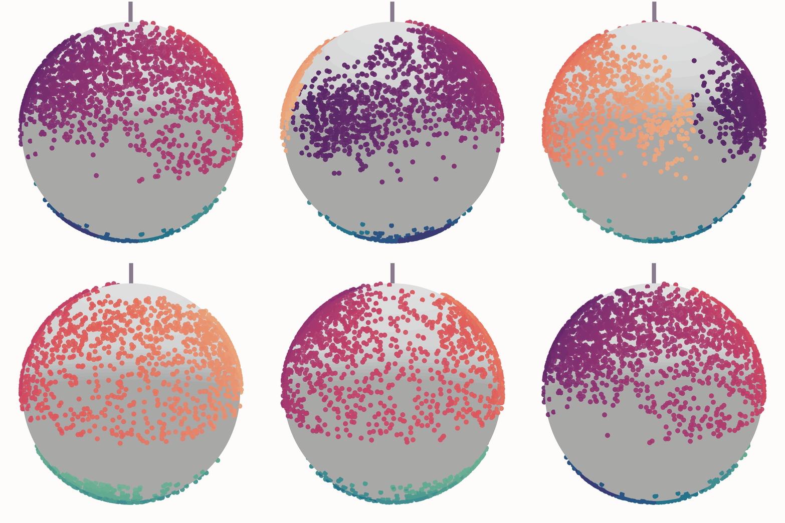
RNA velocity in the Ouroboros Sphere¶

It is possible to have scVelo infer RNA velocity and to output the velocity vectors onto the sphere.

Unfourtunately scVelo is a tricky package that doesn't always play nice with other packages, so you will need a new, specific environment for this purpose.

Also note that scVelo requires the presence of spliced and unspliced counts in your adata.layers().

For more information on scVelo see their tutorial: [https://scvelo.readthedocs.io/en/stable/getting_started.html]

Velocity environment¶

Dependencies

pandas
anndata
scvelo = 0.2.3
scanpy = 1.8.2

To create run:

conda create -n velocity_env python=3.10
conda activate velocity_env

mamba install -c conda-forge -c bioconda "scvelo>=0.2.3" "scanpy>=1.8.2" pandas anndata scikit-learn "numpy<1.24" "pynndescent>=0.5.13"

Then if you want to run this in a jupyter notebook like we do here:

mamba install -c conda-forge ipykernel
python -m ipykernel install --user --name <your_env> --display-name "Python (<your_env>)"

In [1]:

Copied!





import anndata as ad
import scanpy as sc
import pandas as pd
import scvelo as scv
import numpy as np
from sklearn.decomposition import PCA
import anndata as ad
import scanpy as sc
import pandas as pd
import scvelo as scv
import numpy as np
from sklearn.decomposition import PCA

Step 1: Read in the dataset you have run Ouroboros on¶

See our Scanpy/python tutorial for earlier steps.

In [2]:

Copied!

# Read in test dataset - subsetted to existing features
adata = ad.read_h5ad('output_example/example.h5ad')
# Read in test dataset - subsetted to existing features
adata = ad.read_h5ad('output_example/example.h5ad')

We found that cell cycle velocity comes out most cleanly when using the Ouroboros feature set, rather than with all genes as is depicted in the scVelo tutorial. This is likely because dataset may have multiple trajectories (i.e. differentiaiton and cell cycle) and focusing in on only cell cycle informative genes helps to isolate the signal from just the cell cycle.

In [3]:

Copied!





#Replace with path to your installation of Ouroboros 
ouroboros_path = '/projects/steiflab/research/hmacdonald/total_RNA/Ouroboros_pypi'
feature_set = pd.read_csv(f'{ouroboros_path}/ouroboros/data/SHAP_feature_set.csv')
feature_set = feature_set.feature_set.tolist()

# Subset to only include feature set genes 
adata_subset = adata[:, adata.var_names.isin(feature_set)].copy()
#Replace with path to your installation of Ouroboros 
ouroboros_path = '/projects/steiflab/research/hmacdonald/total_RNA/Ouroboros_pypi'
feature_set = pd.read_csv(f'{ouroboros_path}/ouroboros/data/SHAP_feature_set.csv')
feature_set = feature_set.feature_set.tolist()

# Subset to only include feature set genes 
adata_subset = adata[:, adata.var_names.isin(feature_set)].copy()

Next read in the z_df with the latent space embeddings - is the output from Ouroboros

In [4]:

Copied!





# Replace with the path to your z_df 
z_df_path = 'output_example/ouroboros_embeddings_pseudotimes.csv'

z_df = pd.read_csv(z_df_path)
z_df = z_df.set_index('Unnamed: 0')
z_df
# Replace with the path to your z_df 
z_df_path = 'output_example/ouroboros_embeddings_pseudotimes.csv'

z_df = pd.read_csv(z_df_path)
z_df = z_df.set_index('Unnamed: 0')
z_df

Out[4]:

	dim1	dim2	dim3	KNN_phase	cell_cycle_pseudotime	south	dormancy_pseudotime	pseudotime_phase
Unnamed: 0
CTGATCCGTCAGACTT_SRX17782706	0.509849	-0.201015	0.836449	S	0.704949	False	NaN	S
GCCCGAAAGTAGTGCG_SRX17782704	-0.625057	-0.720759	0.299685	G1	0.008879	False	NaN	G1
CCGATGGTCTGATGGT_SRX17782709	-0.292811	-0.886395	0.358562	G2M	0.945957	False	NaN	G2M
CCTCTCCGTTATGTCG_SRX17782704	-0.206861	0.711044	-0.672031	G0	NaN	True	-0.345836	Light_dormancy
AGCGTATGTCTACACA_SRX17782704	0.384594	0.881948	-0.272496	G1-G0 transition	NaN	True	-0.292188	Light_dormancy
...	...	...	...	...	...	...	...	...
TTGTGTTAGCGACAGT_SRX17782709	-0.512673	0.460938	-0.724363	G0	NaN	True	-0.359634	Light_dormancy
ACTGTCCAGTCCTACA_SRX17782709	-0.987645	-0.029321	0.153939	G1	0.140454	False	NaN	G1
TCGCTCAAGCACTCAT_SRX17782706	-0.126240	0.891869	-0.434319	G0	NaN	True	-0.244472	Light_dormancy
GAGTGAGGTATCGTTG_SRX17782709	0.205586	0.704122	-0.679666	G0	NaN	True	-0.429172	Mid_dormancy
TTCGGTCTCGAGCCTG_SRX17782706	0.555647	0.226397	0.800001	S	0.583599	False	NaN	S

400 rows × 8 columns

ScVelo typically works on the dimensions of a UMAP embedding in adata.obsm. To make it accept the latent space instead, we just have to trick it by setting adata.obsm['X_umap'] to be our latent space instead of a UMAP embedding, and then scVelo can run as it normally would.

In [5]:

Copied!

latent_space = z_df[['dim1', 'dim2', 'dim3']].values 

# Set X_umap to be our latent space instead of a UMAP 

adata.obsm['X_umap'] = latent_space
latent_space = z_df[['dim1', 'dim2', 'dim3']].values 

# Set X_umap to be our latent space instead of a UMAP 

adata.obsm['X_umap'] = latent_space

In [6]:

Copied!





# Then scVelo can be run as it normally would be on the adata
## For more info on scVelo see their tutorial: [https://scvelo.readthedocs.io/en/stable/getting_started.html]
vel = adata.copy()
scv.pp.moments(vel, n_neighbors = 20, use_highly_variable = False)
scv.tl.velocity(vel, mode='stochastic')
scv.tl.velocity_graph(vel)
scv.pl.velocity_embedding_stream(vel, basis='umap', title = 'RNA velocity')
# Then scVelo can be run as it normally would be on the adata
## For more info on scVelo see their tutorial: [https://scvelo.readthedocs.io/en/stable/getting_started.html]
vel = adata.copy()
scv.pp.moments(vel, n_neighbors = 20, use_highly_variable = False)
scv.tl.velocity(vel, mode='stochastic')
scv.tl.velocity_graph(vel)
scv.pl.velocity_embedding_stream(vel, basis='umap', title = 'RNA velocity')

Normalized count data: X, spliced, unspliced.

/tmp/ipykernel_1868480/3661863632.py:4: DeprecationWarning: Automatic neighbor calculation is deprecated since scvelo==0.4.0 and will be removed in a future version of scVelo. Please compute neighbors first with Scanpy.
  scv.pp.moments(vel, n_neighbors = 20, use_highly_variable = False)
/projects/pangen/analysis/hmac/applications/miniconda3/envs/velocity_env/lib/python3.10/site-packages/scvelo/preprocessing/moments.py:71: DeprecationWarning: `neighbors` is deprecated since scvelo==0.4.0 and will be removed in a future version of scVelo. Please compute neighbors with Scanpy.
  neighbors(
/projects/pangen/analysis/hmac/applications/miniconda3/envs/velocity_env/lib/python3.10/site-packages/scvelo/preprocessing/neighbors.py:233: DeprecationWarning: Automatic computation of PCA is deprecated since scvelo==0.4.0 and will be removed in a future version of scVelo. Please compute PCA with Scanpy first.
  _set_pca(adata=adata, n_pcs=n_pcs, use_highly_variable=use_highly_variable)

computing neighbors
    finished (0:00:43) --> added 
    'distances' and 'connectivities', weighted adjacency matrices (adata.obsp)
computing moments based on connectivities
    finished (0:00:01) --> added 
    'Ms' and 'Mu', moments of un/spliced abundances (adata.layers)
computing velocities
    finished (0:00:08) --> added 
    'velocity', velocity vectors for each individual cell (adata.layers)
computing velocity graph (using 1/144 cores)
WARNING: Unable to create progress bar. Consider installing `tqdm` as `pip install tqdm` and `ipywidgets` as `pip install ipywidgets`,
or disable the progress bar using `show_progress_bar=False`.
    finished (0:00:00) --> added 
    'velocity_graph', sparse matrix with cosine correlations (adata.uns)
computing velocity embedding
    finished (0:00:00) --> added
    'velocity_umap', embedded velocity vectors (adata.obsm)

No description has been provided for this image

We can then take the velocity vectors straight from the adata itself:

In [7]:

Copied!

vel_df = pd.DataFrame(vel.obsm['velocity_umap'], columns = ['dim1', 'dim2', 'dim3'], index = vel.obs.index)

vel_df.to_csv('output_example/example_velocity_df.csv')
vel_df = pd.DataFrame(vel.obsm['velocity_umap'], columns = ['dim1', 'dim2', 'dim3'], index = vel.obs.index)

vel_df.to_csv('output_example/example_velocity_df.csv')

We can't access Ouroboros functions like plot_sphere() here because scVelo conflicts with some of the Ouroboros dependencies.

So, to plot these vectors onto the sphere, you can save the velocity dataframe to a csv, and load them into a new notebook using the ouroboros_env kernal.

Here we switch to our ouroboros_env to run this code:

In [1]:

Copied!





import scanpy as sc
import anndata as ad
import numpy as np
import ouroboros as obo
import importlib_resources as resources
import seaborn as sns
import pandas as pd
import cartopy.crs as ccrs

# this is just for the tutorial rendering
from IPython.display import IFrame

import scanpy as sc
import anndata as ad
import numpy as np
import ouroboros as obo
import importlib_resources as resources
import seaborn as sns
import pandas as pd
import cartopy.crs as ccrs

# this is just for the tutorial rendering
from IPython.display import IFrame

In [2]:

Copied!

# Read in your latent space embeddings - Replace with the path to your z_df 
z_df_path = 'output_example/ouroboros_embeddings_pseudotimes.csv' 

z_df = pd.read_csv(z_df_path)
z_df = z_df.set_index('Unnamed: 0')
print(z_df.head())
# Read in your latent space embeddings - Replace with the path to your z_df 
z_df_path = 'output_example/ouroboros_embeddings_pseudotimes.csv' 

z_df = pd.read_csv(z_df_path)
z_df = z_df.set_index('Unnamed: 0')
print(z_df.head())

                                  dim1      dim2      dim3         KNN_phase  \
Unnamed: 0                                                                     
CTGATCCGTCAGACTT_SRX17782706  0.509849 -0.201015  0.836449                 S   
GCCCGAAAGTAGTGCG_SRX17782704 -0.625057 -0.720759  0.299685                G1   
CCGATGGTCTGATGGT_SRX17782709 -0.292811 -0.886395  0.358562               G2M   
CCTCTCCGTTATGTCG_SRX17782704 -0.206861  0.711044 -0.672031                G0   
AGCGTATGTCTACACA_SRX17782704  0.384594  0.881948 -0.272496  G1-G0 transition   

                              cell_cycle_pseudotime  south  \
Unnamed: 0                                                   
CTGATCCGTCAGACTT_SRX17782706               0.704949  False   
GCCCGAAAGTAGTGCG_SRX17782704               0.008879  False   
CCGATGGTCTGATGGT_SRX17782709               0.945957  False   
CCTCTCCGTTATGTCG_SRX17782704                    NaN   True   
AGCGTATGTCTACACA_SRX17782704                    NaN   True   

                              dormancy_pseudotime pseudotime_phase  
Unnamed: 0                                                          
CTGATCCGTCAGACTT_SRX17782706                  NaN                S  
GCCCGAAAGTAGTGCG_SRX17782704                  NaN               G1  
CCGATGGTCTGATGGT_SRX17782709                  NaN              G2M  
CCTCTCCGTTATGTCG_SRX17782704            -0.345836   Light_dormancy  
AGCGTATGTCTACACA_SRX17782704            -0.292188   Light_dormancy

In [3]:

Copied!





# Read in your velocity vectors for those embeddings 
vel_df = pd.read_csv('output_example/example_velocity_df.csv')
vel_df = vel_df.set_index('Unnamed: 0')
print(vel_df.head())
# Read in your velocity vectors for those embeddings 
vel_df = pd.read_csv('output_example/example_velocity_df.csv')
vel_df = vel_df.set_index('Unnamed: 0')
print(vel_df.head())

                                  dim1      dim2      dim3
Unnamed: 0                                                
CTGATCCGTCAGACTT_SRX17782706 -0.014624 -0.027485  0.004248
GCCCGAAAGTAGTGCG_SRX17782704 -0.000823  0.026368 -0.039530
CCGATGGTCTGATGGT_SRX17782709 -0.008505  0.004189 -0.013428
CCTCTCCGTTATGTCG_SRX17782704 -0.020949 -0.001416 -0.006240
AGCGTATGTCTACACA_SRX17782704 -0.037803  0.013704 -0.037323

In [4]:

Copied!

# Plot the sphere as before, but give the velocity vector df to the parameter velocity to have it plot the vectors too 
fig = obo.plot_sphere(z_df, colour_by='KNN_phase', velocity=vel_df, show=False, savefig = 'output_example/example_sphere_with_velocity.html')
IFrame(src="../output_example/example_sphere_with_velocity.html", width="100%", height=600)

# Plot the sphere as before, but give the velocity vector df to the parameter velocity to have it plot the vectors too 
fig = obo.plot_sphere(z_df, colour_by='KNN_phase', velocity=vel_df, show=False, savefig = 'output_example/example_sphere_with_velocity.html')
IFrame(src="../output_example/example_sphere_with_velocity.html", width="100%", height=600)

Out[4]:

We can also plot RNA velocity vectors on the robinson/map projection. * sometimes the scale of the arrows gets funky so you may have to adjust the 'scale' parameter

In [5]:

Copied!





obo.plot_robinson_projection(
    z_df, 
    colour_by = 'KNN_phase',
    velocity_df=vel_df, 
    palette=None, 
    ref=None,
    central_longitude=80, 
    title="Robinson projection", 
    alpha=0.7,
    scale=3
    
)
obo.plot_robinson_projection(
    z_df, 
    colour_by = 'KNN_phase',
    velocity_df=vel_df, 
    palette=None, 
    ref=None,
    central_longitude=80, 
    title="Robinson projection", 
    alpha=0.7,
    scale=3
    
)

RNA velocity in the Ouroboros Sphere¶

Velocity environment¶

Step 1: Read in the dataset you have run Ouroboros on¶

Ouroboros

Navigation

Table Of Contents