API Reference
This page documents the main functions available when importing ouroboros as a Python package.
run_ouroboros(data, data_type, species='human', outdir='.')
Description:
Runs the full Ouroboros pipeline on either .h5ad or .csv input and outputs latent embeddings, pseudotime values, and plots.
Parameters:
| Name | Type | Description |
|---|---|---|
data |
str or AnnData |
Path to file or pre-loaded AnnData object |
data_type |
str |
Either 'h5ad' or 'csv' |
species |
str |
'human' or 'mouse' (mouse gene names are auto-mapped) |
outdir |
str |
Directory to write output CSVs and HTML plots |
Returns:
pandas.DataFrame — DataFrame containing 3D coordinates and predicted states for each cell.
check_genes(adata)
Description: Checks if any feature genes are missing from a test anndata object. Returns a list of missing genes
Parameters:
| Parameter | Type | Description |
|---|---|---|
adata |
AnnData |
Test anndata object with adata.var_names in HUGO formatting (e.x. CCNE1) |
read_in_features()
Description: Reads in all Ouroboros feature genes. No input necessary. Returns a list of genes.
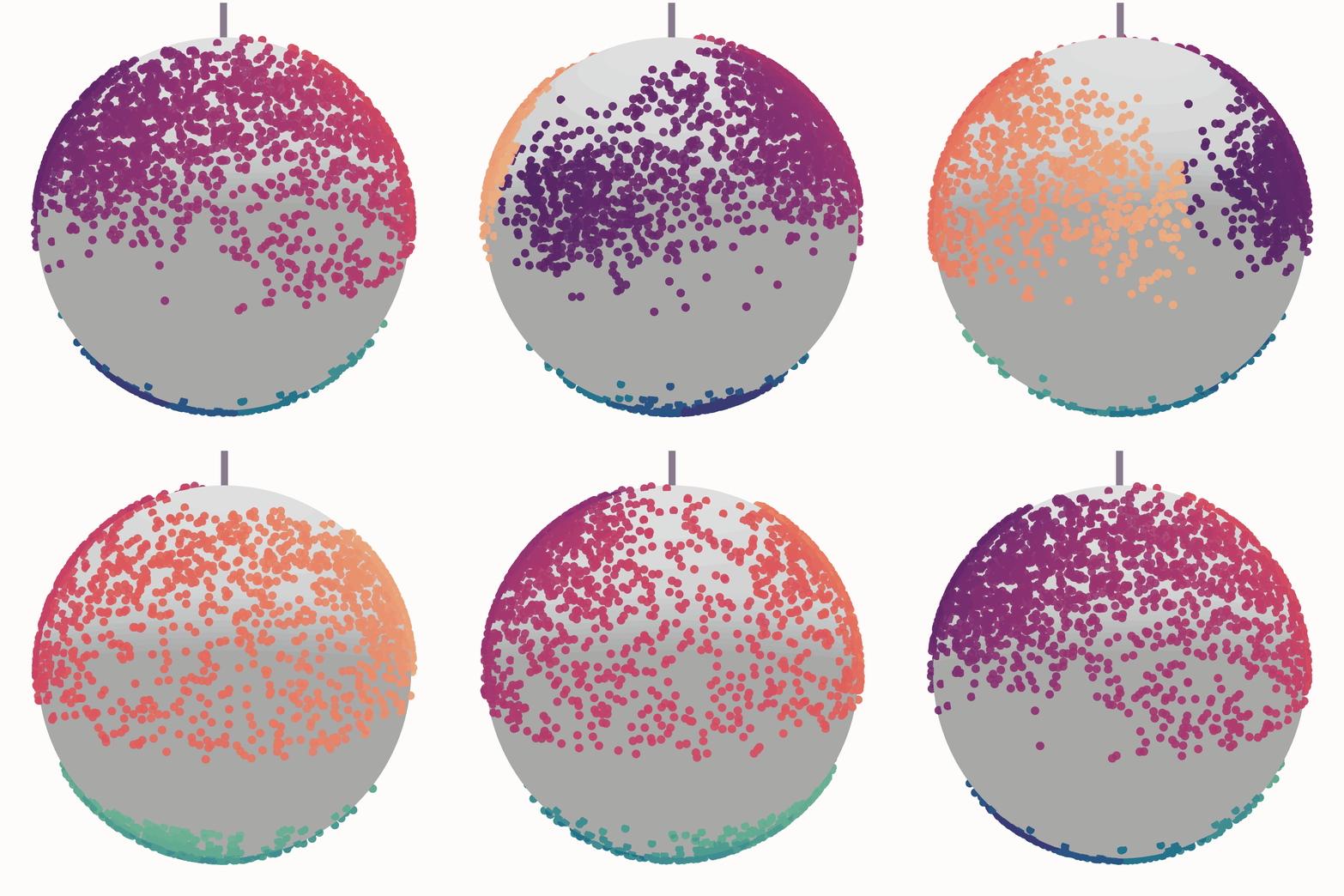
plot_sphere(z_df, colour_by = 'KNN_phase', palette = None, ref = None, velocity = None, marker_size = 2, cycle_pole = [0, 0, 1], savefig = None, show = False)
Description:
Generates an interactive 3D spherical projection of the Ouroboros latent space.
Example usage
plot_sphere(
    z_df: pd.DataFrame,
    colour_by: str = 'KNN_phase',
    palette: dict | str = None,
    ref: pd.DataFrame = None,
    velocity: pd.DataFrame = None,
    marker_size: int = 2,
    cycle_pole: list[float] = [0,0,1],
    savefig: str = None,
    show: bool = False
)
Parameters:
| Parameter | Type | Description |
| ------------- | -------------------- | ----------- |
| z_df | DataFrame | Cell dataframe with 3D spherical coordinates (dim1, dim2, dim3) and metadata columns such as phase labels or pseudotime. |
| colour_by | str | Column in z_df to colour points by (e.g. 'KNN_phase', 'cell_cycle_pseudotime', 'dormancy_depth'). |
| palette | dict or str | Optional colour map: a dictionary for categorical data (e.g. {'G1': 'blue', 'G2M': 'green'}), or a colormap name (e.g. 'mako', 'rocket_r') for continuous data. If None, a sensible default is used. |
| ref | DataFrame or str | Optional reference cells to overlay as faint points. Use 'default' to show the training embeddings from the paper (only valid if you did not retrain the model). If you retrained, pass your own reference DataFrame with columns dim1, dim2, dim3 and phase. Use None to show no reference points. |
| velocity | DataFrame | Optional velocity vectors with columns dim1, dim2, dim3. |
| marker_size | int | Size of scatter points. |
| savefig | str | If provided, saves the plot as an HTML file at this path. |
| show | bool | Whether to display the figure. |
def plot_gene_sphere(z_df, adata, gene_name, layer=None, ref=None, velocity=None, show=False, outpath=None, cycle_pole=reference_CC_pole_point)
Description:
Generates an interactive 3D spherical projection of the Ouroboros latent space, coloured by the expression of a given gene.
Example usage
plot_gene_sphere(
    z_df: pd.DataFrame,
    adata: anndata.AnnData,
    gene_name: str,
    layer: str = None,
    ref: pd.DataFrame = None,
    ref_color: str = 'putative_phase_transition',
    ref_pal: dict = phase_pal_transition,
    velocity: pd.DataFrame = None,
    show: bool = False,
    outpath: str = None,
    cycle_pole: list[float] = reference_CC_pole_point
)
Parameters:
| Parameter | Type | Description |
|---|---|---|
z_df |
DataFrame |
DataFrame containing embedded cell coordinates (dim1, dim2, dim3) and metadata columns. |
adata |
AnnData |
The original single-cell data object containing expression values. |
gene_name |
str |
Gene to plot. Must exist in adata.var_names. |
layer |
str, optional |
Name of the .layers slot in adata to use (e.g. "log_counts"). Defaults to .X. |
ref |
DataFrame, optional |
Optional reference cells to overlay as faint points. Use 'default' to show the training embeddings from the paper (only valid if you did not retrain the model). If you retrained, pass your own reference DataFrame with columns dim1, dim2, dim3 and phase. Use None to show no reference points. |
velocity |
DataFrame, optional |
Optional velocity vectors (same shape as z_df) with dim1, dim2, dim3. See plot_velocity for more information. |
show |
bool, default False |
Whether to display the plot interactively in a Jupyter notebook. |
outpath |
str, optional |
If provided, saves the interactive Plotly figure as HTML. |
cycle_pole |
list[float] |
A 3D point marking the known cell cycle pole for axis. If you did not retrain model, the reference is correct and you do not need to supply it. If you did retrain the model, you can either provide 'None' and not plot it, or use find_cycle_pole to identify |
sphere_snapshot(lat, lon, z_df, colour_by='KNN_phase', palette=None, radius = 1.2, ref_embed = None, vel_df = None, save_as_png=True, cycle_pole = [0, 0, 1])
Description: Produces a png of the sphere at a given latitude and longtiude and writes it to a given output path.
Example usage:
sphere_snapshot(
    lat: int,
    long: int,
    z_df: pd.DataFrame,
    colour_by: str,
    radius: float,
    gene_name: str,
    layer: str = None,
    ref_embed: pd.DataFrame = None,
    vel_df: pd.DataFrame = None,
    save_as_png: str # ex. /path/to/output/png
    cycle_pole: list[float] = [0,0,1]
)
Parameters:
| Parameter | Type | Description |
| ------------- | ------------------------- | ----------------------------------------------------------------------------------------------------------------------------------------- |
| lat | int | Latitude angle (in degrees) to position the camera viewpoint. Must be in [-90, 90]. |
| lon | int | Longitude angle (in degrees) to position the camera viewpoint. Must be in [0, 360]. |
| z_df | DataFrame | DataFrame containing spherical embedding coordinates (dim1, dim2, dim3) and metadata. |
| colour_by | str | Column in z_df to color points by (e.g., 'KNN_phase', 'cell_cycle_pseudotime'). |
| radius | float, optional | Distance from the sphere center to the virtual camera. Controls zoom level. |
| palette | dict or str, optional | Color palette. Use a dictionary for categorical values or a colormap name (e.g., 'mako') for continuous values. |
| ref | DataFrame, optional | Optional reference cells to overlay as faint points. Use 'default' to show the training embeddings from the paper (only valid if you did not retrain the model). If you retrained, pass your own reference DataFrame with columns dim1, dim2, dim3 and phase. Use None to show no reference points. |
| vel_df | DataFrame, optional | Optional velocity vectors with columns dim1, dim2, dim3. Drawn as arrows and cones. |
| save_as_png | str, optional | Path to save the image as a PNG. If None, the image is not saved. |
| showlegend | bool, default False | Whether to display the legend in the plot. |
| cycle_pole | list[float], optional | 3D vector indicating the cell cycle pole. Defaults to [0, 0, 1]. If you haven't rotated the sphere the cycle pole will be off. |
convert_to_human_genes()
Converts mouse gene symbols to their human orthologs (HGNC symbols). Ouroboros runs this automatically when species='mouse'. It's documented here in case you need it elsewhere, for example to compare mouse and human datasets.
convert_to_human_genes(data: ad.AnnData | pd.DataFrame) -> ad.AnnData | pd.DataFrame
| Parameter | Type | Description |
|---|---|---|
data |
AnnData or DataFrame |
Mouse expression data. For AnnData, gene symbols must be in var_names. For a DataFrame, cells are rows and gene symbols are columns. |
Returns: the same type as the input (AnnData or DataFrame), with human gene symbols as the gene names.
What it does:
- Keeps only mouse genes with a known human ortholog. Genes without an ortholog are dropped.
- Renames each mouse gene to its human ortholog.
- Sums duplicates. If several mouse genes map to the same human gene (e.g. mouse paralogs), their counts are added together into a single human gene.
Notes:
- Use raw counts. Duplicate genes are combined by summing, which is appropriate for counts but not for log-normalised or scaled values. Normalise after converting.
- Gene symbols must match exactly, including case (e.g.
Top2a, notTOP2Aor an Ensembl ID). - For
AnnDatainput, onlyXandobsare kept. Gene metadata (varcolumns),layers,obsm(e.g. UMAP),varmandunsare not carried over. The returned matrix is dense. - Raises a
ValueErrorif none of the input genes match a known mouse gene.
Example:
import scanpy as sc
import ouroboros as obo

adata_mouse = sc.read_h5ad("mouse_counts.h5ad")
adata_human = obo.convert_to_human_genes(adata_mouse)

print(adata_mouse.n_vars, "→", adata_human.n_vars, "genes")
adata_human.var_names[:5]
plot_robinson_projection(z_df, colour_by, velocity_df=None, palette=None, ref=None, central_longitude=80, title="", alpha=0.7, scale=10, save_fig=None, rasterize=True, show=True)
Description:
Projects 3D spherical coordinates onto a 2D Robinson map with flexible coloring by categorical or continuous metadata. Cartesian coordinates (dim1, dim2, dim3) are converted to longitude/latitude and drawn on a Robinson projection; coloring is auto-detected as continuous or categorical, NA values are shown in grey, and an optional reference set can be drawn as faint background points. Used for interpreting global cell state structure or transitions in a biologically interpretable planar projection.
Example usage:
plot_robinson_projection(
    z_df=embedding_df,
    colour_by='cell_cycle_pseudotime',
    velocity_df=velocity_df,
    palette='rocket_r',
    ref=reference_df,
    title="Differentiation Trajectory",
    scale=15,
    save_fig="robinson.png"
)
Parameters:
| Parameter | Type | Description |
| ------------------- | ------------------------- | ----------------------------------------------------------------------------------------------------------------------------------------------------- |
| z_df | DataFrame | DataFrame containing 3D spherical embedding coordinates (dim1, dim2, dim3) and associated metadata for coloring. |
| colour_by | str | Column in z_df to color by. Automatically handled as categorical (e.g., 'KNN_phase') or continuous (e.g., 'cell_cycle_pseudotime'). |
| velocity_df | DataFrame, optional | Optional RNA velocity DataFrame with dim1, dim2 columns representing directional flow vectors, drawn as quiver arrows. |
| palette | dict or str, optional | Custom palette: a dict mapping labels to colors for categorical data, or a colormap name (e.g., 'mako', 'viridis') for continuous data. If None, a colormap is auto-selected (rocket_r for cell_cycle_pseudotime, mako for dormancy_pseudotime, else viridis; tab20/phase_pal_transition for categorical). |
| ref | DataFrame, optional | Optional reference cells to overlay as faint points. Use 'default' to show the training embeddings from the paper (only valid if you did not retrain the model). If you retrained, pass your own reference DataFrame with columns dim1, dim2, dim3 and phase. Use None to show no reference points. |
| central_longitude | int, default 80 | Longitude (in degrees) to center the Robinson projection. |
| title | str, optional | Title of the plot. |
| alpha | float, default 0.7 | Transparency of the primary data points. |
| scale | float, default 10 | Scale of the velocity vector arrows (larger values produce shorter arrows). |
| save_fig | str, optional | File path to save the figure to (300 dpi, tight bounding box). If None, the figure is not saved. |
| rasterize | bool, default True | Whether to rasterize the scatter and quiver layers, keeping file sizes small when plotting many points while leaving axes/text as vectors. |
| show | bool, default True | Whether to display the figure with plt.show(). |
📘 For full tutorials, see the Python Tutorial.